개발 환경 : pycharm-community-2020.2 (무료 에디션)
Anaconda, python3.7, Windows 10
ANN : 생체신경망 구조와 유사하게 은닉 계층을 포함하는 인공신경망 기술이다.
입력계층 -> 은닉계층 -> 출력계층 으로 구성되고 각 계층은 순서대로 입력노드, 은닉노드, 출력노드를 포함한다.
분류(ANN) : 입력 정보를 클래스별로 분류하는 방식
- 해당 입력이 어느 클래스에 속하는지 결정한다.
- 분류 할 클래스 수만큼 출력노드를 만드는 방법이 효과적이다.
- ANN을 구성하는 가중치의 학습은 예측값의 목표값에 대한 오차를 역방향으로 되돌리며 이루어짐으로 '오차역전파' 라고 한다.
필기체를 구분하는 분류 ANN 구현
1단계 패키지 불러오기
from keras import layers, models
layers : 계층을 만드는 모듈
models : 각 layer을 연결해 신경망 모델을 만든 후 컴파일하고 학습시키는 역할, 학습 후 평가도 진행한다.
2단계 분류 ANN에 필요한 파라미터 설정
Nin : 입력 계층 노드 수
Nh : 은닉 계층 노드 수
number_of_class : 출력값이 가질 클래스 수
Nout : 출력 계층 노드 수
3단계 분류 ANN 모델 구현
케라스는 인공지능 모델을 연쇄방식과 분산방식으로 구현할 수 있다.
구현하는 방식도 함수형과 객체지향형이 있다.
활성화 함수 'relu' : f(x)=max(x,0)
(1) 분산방식 모델링 함수형 구현
def ANN_models_func(Nin, Nh, Nout):
    x= layers.Input(shape=(Nin,)) #입력계층
    h= layers.Activation('relu')(layers.Dense(Nh)(x)) #은닉계층
    y= layers.Activation('softmax')(layers.Dense(Nout)(h)) #출력계층
    model= models.Model(x,y)
    model.compile(loss='categorical_crossentropy',optimizer='adam',metrics=['accuracy'])
    return model
layers.Dense(Nh)(x) : 노드가 Nh인 은닉 계층을 지정하고 x를 입력으로 받아들인다.
(2) 연쇄방식 모델링 함수형 구현
def ANN_seq_func(Nin, Nh, Nout):
    model = models.Sequential() #모델 초기화
    model.add(layers.Dense(Nh, activation='relu', input_shape=(Nin,))) #입력, 은닉계층 설정
    model.add(layers.Dense(Nout, activation='softmax'))
    model.compile(loss='categorical_crossentropy',optimizer='adam',metrics=['accuracy'])
    return model
입력 계층은 layers.Input 함수로 지정한다.
입력 노드 Nin개는 Nh로 구성된 은닉계층으로 보내진다.
add 함수로 계층의 추가가 가능하다는 장점이 있다.
(3) 분산방식 모델링 객체지향형 구현 : 복잡한 인공신경망 기술로 ANN 코드의 재사용성을 높인다.
(4) 연쇄방식 모델링 객체지향형 구현
class ANN_seq_class(models.Sequential):
    def __init__(self, Nin, Nh, Nout):
        super().__init__()
        self.add(layers.Dense(Nh, activation='relu', input_shape=(Nin,)))
        self.add(layers.Dense(Nout, activation='softmax'))
        self.compile(loss='categorical_crossentropy',optimizer='adam',metrics=['accuracy'])
4단계 학습과 성능 평가용 데이터 불러오기
MNIST 데이터셋을 사용 - 6만 건의 필기체 숫자를 모은 공개 데이터
먼저, 데이터를 불러오는 라이브러리를 가져온다.
import numpy as np
from keras import datasets #mnist ()
from keras.utils import np_utils # to_categorical ()
5단계 학습 및 검증
불러온 데이터(load_data)를 변수에 저장한다.
X_ 와 y_ 를 이니셜로 하는 입력과 출력 변수에 각각 저장
_train : 학습에 사용하는 데이터 저장
_test : 성능 평가에 사용하는 데이터 저장
(X_train, y_train), (X_test, y_test) = datasets.mnist.load_data()
0부터 9까지의 숫자로 구성된 출력값을 0과 1로 표현되는 벡터로 변환
Y_train= np_utils.to_categorical(y_train)
Y_test= np_utils.to_categorical(y_test)
3차원 데이터(픽셀, 이미지)를 2차원으로 조정
학습 데이터셋에 샘플이 L개, 따라서 L * W * H 와 같은 모양의 텐서로 저장되어 있다.
-1 은 행렬의 행을 자동으로 설정하게 만든다.
L, W, H= X_train.shape
X_train=X_train.reshape(-1, W * H)
X_test=X_test.reshape(-1, W * H)
ANN 최적화를 위해 아규먼트 정규화
0~255 사이의 정수 입력값을 255로 나누어 0~1사이의 실수로 바꾼다.
X_train = X_train/255.0
X_test = X_test/255.0
학습 결과 그래프 구현
그래프를 그리는 라이브러리 plt
import matplotlib.pyplot as plt
def plot_loss(history): #손실을 그리는 함수
plt.plot(history.history['loss'])
plt.plot(history.history['val_loss']) #검증
plt.title('Model Loss')
plt.ylabel('Loss')
plt.xlabel('Epoch')
plt.legend(['Train','Test'], loc=0)
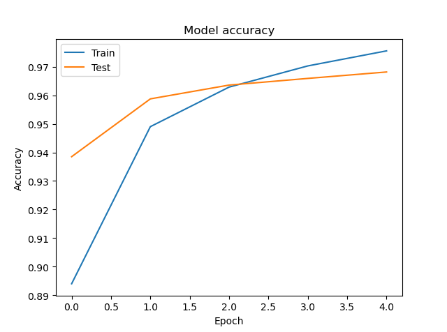
def plot_acc(history): #정확도를 그리는 함수
plt.plot(history.history['accuracy'])
plt.plot(history.history['val_accuracy'])
plt.title('Model accuracy')
plt.ylabel('Accuracy')
plt.xlabel('Epoch')
plt.legend(['Train','Test'], loc=0) #각 라인의 표식 표시
6단계 학습 및 성능 분석
X_train, Y_train : 학습에 사용할 입력, 출력데이터
batch_size : 한 데이터를 얼마씩 나눠서 넣을지를 지정
validation_split=0.2 : 학습 데이터의 20%만큼 성능 검증에 사용한다는 의미
def main():
    Nin= 784 #입력 Nin은 길이가 784인 데이터
    Nh=100 #은닉노드수
    number_of_class=10
    Nout= number_of_class

    model= ANN_seq_class(Nin, Nh, Nout)
    (X_train, Y_train), (X_test, Y_test) = Data_func()

    history= model.fit(X_train, Y_train, epochs=5, batch_size=100, validation_split=0.2)
    performance_test= model.evaluate(X_test, Y_test, batch_size=100)
    print('test Loss and accurancy ->',performance_test)
전체코드
from keras import layers, models

# 연쇄방식 모델링 객체지향형 구현
class ANN_seq_class(models.Sequential):
    def __init__(self, Nin, Nh, Nout):
        super().__init__()
        self.add(layers.Dense(Nh, activation='relu', input_shape=(Nin,)))
        self.add(layers.Dense(Nout, activation='softmax'))
        self.compile(loss='categorical_crossentropy',optimizer='adam',metrics=['accuracy'])

#분류 ANN에 사용할 데이터 불러오기
import numpy as np
from keras import datasets #mnist
from keras.utils import np_utils #to_categorical

def Data_func():
    (X_train, y_train), (X_test, y_test)= datasets.mnist.load_data()
    # 출력값을 벡터로 변환
    Y_train =np_utils.to_categorical(y_train)
    Y_test= np_utils.to_categorical(y_test)
    #3차원 데이터(픽셀, 이미지)를 2차원으로 조정
    L, W, H= X_train.shape
    X_train=X_train.reshape(-1, W * H)
    X_test=X_test.reshape(-1, W * H)
    # ANN최적화를 위해 아규먼트 정규화
    X_train = X_train/255.0
    X_test = X_test/255.0
    return (X_train, Y_train), (X_test, Y_test)

# 분류 ANN 학습 결과 그래프 구현
import matplotlib.pyplot as plt

def plot_loss(history): #손실을 그리는 함수
    plt.plot(history.history['loss'])
    plt.plot(history.history['val_loss']) #검증
    plt.title('Model Loss')
    plt.ylabel('Loss')
    plt.xlabel('Epoch')
    plt.legend(['Train','Test'], loc=0)

def plot_acc(history): #정확도를 그리는 함수
    plt.plot(history.history['accuracy'])
    plt.plot(history.history['val_accuracy'])
    plt.title('Model accuracy')
    plt.ylabel('Accuracy')
    plt.xlabel('Epoch')
    plt.legend(['Train','Test'], loc=0) #각 라인의 표식 표시

# 분류 ANN 학습 및 성능분석
def main():
    Nin= 784 #입력 Nin은 길이가 784인 데이터
    Nh=100 #은닉노드수
    number_of_class=10
    Nout= number_of_class

    #모델 인스턴스 생성, 데이터를 불러오기
    model= ANN_seq_class(Nin, Nh, Nout)
    (X_train, Y_train), (X_test, Y_test) = Data_func()

    history= model.fit(X_train, Y_train, epochs=5, batch_size=100, validation_split=0.2)
    performance_test= model.evaluate(X_test, Y_test, batch_size=100)
    print('test Loss and accurancy ->',performance_test)

    plot_loss(history)
    plt.show()

    plot_acc(history)
    plt.show()

# run code
if __name__ == '__main__':
    main()
콘솔 결과 확인

손실 : 0.1043
정확도 : 0.9682
plot_loss 그래프 출력

plot_acc 그래프 출력
책 그대로 타이핑 했는데 오류가 있었다. - 다운받은 예제소스도 마찬가지
'acc' 이게 오류임을 콘솔에서 확인하고 같은 반 선배한테 물어보니까 동일하게 'accurancy' 로 해야한다는 것을 알게 되었다.
참고 : 코딩셰프의 3분 딥러닝 케라스맛
'Keras Deep Learning' 카테고리의 다른 글
| 컬러 이미지를 분류하는 DNN 구현 실습 (0) | 2020.08.20 |
|---|---|
| 필기체를 분류하는 DNN 구현 실습 (0) | 2020.08.19 |
| DNN(심층신경망) 개념, 경사도 소실 문제 & ReLU 활성화 함수 (0) | 2020.08.19 |
| 회귀 ANN(인공신경망) 실습 (0) | 2020.08.19 |
| Keras 시작하기 - 케라스로 인공신경망 구축 실습 (0) | 2020.08.18 |


